Crafting Personalized Compounding Models for Financial Independence

Introduction to Personalized Compounding Models

Financial independence (FI) requires precise planning, and generic calculators often fall short. Crafting personalized compounding models allows you to align projections with your unique contribution rates, timelines, and risk tolerance. This approach emphasizes accuracy through DIY methods that adapt to individual circumstances rather than one-size-fits-all apps. Compounding remains the foundation of wealth building. By modeling it yourself, you gain control over variables that matter most to your FI journey. Many aspiring retirees discover that off-the-shelf tools overlook nuances like irregular income streams or specific lifestyle inflation patterns, leading to projections that feel disconnected from reality.

Personalized models empower users to simulate multiple life scenarios, from career changes to market downturns, ensuring the path to FI feels achievable and grounded. This depth of customization transforms abstract goals into concrete, trackable plans that evolve with you.

Core Formulas for Compounding Calculations

The future value of a series of contributions uses the formula: FV = P * (((1 + r)^n - 1) / r) * (1 + r), where P is the periodic payment, r is the periodic rate, and n is the number of periods. For lump sums, apply FV = PV * (1 + r)^n. Personalization comes from adjusting these inputs to match your expected returns, inflation adjustments, and withdrawal rates. Always incorporate real returns by subtracting inflation. This ensures projections reflect purchasing power in retirement. Break down the formula step by step in your model by creating helper cells that calculate periodic rates from annual assumptions, making it easier to tweak variables without errors.

Advanced users extend these formulas to include dividend reinvestment or variable contribution schedules. For instance, separate the growth component from contribution growth to isolate the true impact of compounding over decades.

Setting Up Your Spreadsheet Step by Step

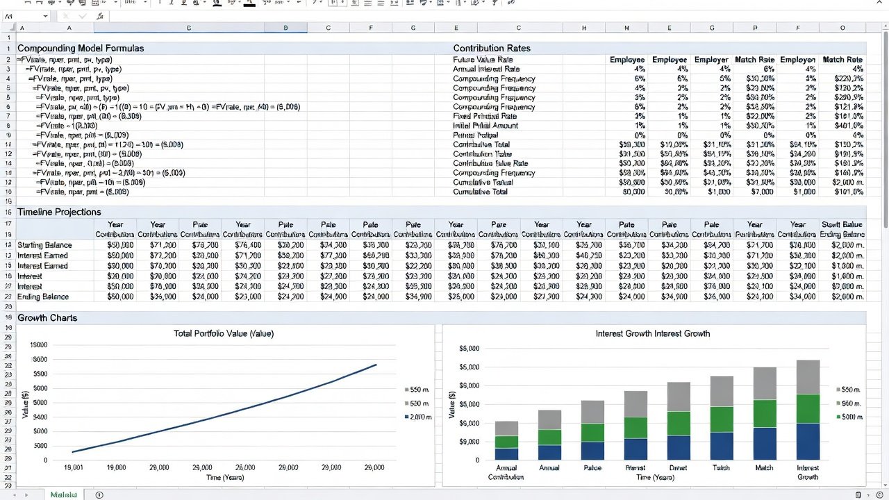
Begin with a new workbook in your preferred tool. Create columns for year, starting balance, annual contribution, expected return rate, ending balance, and cumulative contributions. Use cell references for all variables so changes propagate automatically. Implement the compounding formula in the ending balance column. Add a separate sheet for sensitivity analysis, testing different return scenarios and contribution increases. Label every input cell clearly and apply data validation to prevent entry mistakes, such as negative rates. Color-code assumptions versus calculated fields for quick visual scanning during reviews.

Next, build a dashboard tab that summarizes key metrics like projected FI date and total nest egg at retirement. Include charts that dynamically update as inputs change, providing immediate visual feedback on how adjustments affect outcomes. Test the setup with a small sample dataset before expanding to full projections.

Key Variable Inputs and Customization

Contribution rates form the heart of personalization. Input your current savings rate and project annual increases tied to income growth. Timelines should reflect your target FI date, with buffers for unexpected delays. Include tax-advantaged account limits where relevant and model side income streams separately. Other inputs include expense inflation rates and safe withdrawal percentages. Test multiple combinations to identify robust paths to independence. Consider incorporating variables for one-time windfalls, such as bonuses or inheritances, by adding dedicated rows that apply compounding only from their receipt date onward.

Account for sequence-of-returns risk by layering different return profiles across accumulation and decumulation phases. This customization reveals how early market volatility can extend your working years or force lifestyle adjustments later.

Accounting for Inflation, Taxes, and Market Volatility

Inflation erodes purchasing power, so apply an annual rate to both expenses and contributions within the model. Taxes complicate projections when mixing taxable and tax-advantaged accounts; create separate columns for pre-tax and after-tax balances. Volatility can be modeled through Monte Carlo-style simulations using random return generators in spreadsheet functions, though simpler versions apply historical standard deviations to stress-test results.

These layers add realism. For example, adjusting for a 3% inflation assumption alongside 2% annual contribution increases shows how real savings power changes over time.

Real-World Numerical Examples

Consider an individual starting with $50,000, contributing $2,000 monthly at a 7% real return over 20 years. The model shows substantial growth driven by consistent additions and compounding. Adjusting the contribution upward by 3% annually accelerates the timeline noticeably. A second example involves a couple with uneven incomes: one partner contributes steadily while the other ramps up after a career shift at year eight. The spreadsheet captures this by allowing variable annual inputs rather than fixed monthly averages.

A third scenario compares aggressive versus conservative portfolios, illustrating how a 2% difference in assumed returns compounds into hundreds of thousands over 25 years. These examples demonstrate why manual models outperform generic tools that cannot accommodate such granular detail.

Manual Models Versus Popular Apps

Spreadsheet models offer full transparency and customization unavailable in most apps. You control every assumption and can integrate personal data like expected inheritances or career changes. Popular tools provide convenience but often use averaged assumptions that overlook your specific goals. Manual approaches require initial effort yet deliver superior accuracy for complex FI plans. They also avoid subscription costs associated with premium app features. Apps may update automatically with market data, but spreadsheets let you decide exactly which data sources to trust and how to weight them.

Common Projection Errors and FAQ

• Overly optimistic returns: Use conservative estimates based on historical averages rather than recent bull markets.
• Ignoring sequence of returns risk: Model different market conditions during withdrawal phases.
• Static contributions: Always include growth assumptions for savings rates.
• Neglecting fees: Deduct estimated expense ratios from expected returns each year.
• Single-point estimates: Run at least three scenarios: base, optimistic, and pessimistic.

Frequently Asked Questions

How often should I update my model? Review inputs quarterly and perform a full revision annually.

What if my actual returns differ from projections? Re-run scenarios with updated rates to adjust contributions or timelines accordingly.

Can I include multiple income sources? Yes, dedicate separate rows or sections for each stream within the spreadsheet.

How do I handle irregular expenses like home repairs? Create a contingency bucket that grows with inflation and draws down only in modeled years.

Is it worth modeling Social Security or pensions? Absolutely, subtract estimated benefits from required portfolio withdrawals to lower the target nest egg.

Actionable Tips for Annual Model Updates in 2026

Schedule a dedicated review each January. Reassess expected returns using recent market data and adjust contribution targets based on the prior year's performance. Incorporate life changes such as new expenses or income sources immediately. Validate formulas remain error-free after each update and compare outputs against your actual portfolio balances. Document all changes in a dedicated notes tab for future reference. This habit ensures your personalized model stays relevant and actionable. Revisit withdrawal rate assumptions every few years as new research on safe rates emerges, and cross-check your asset allocation against current economic conditions to keep the model aligned with reality.

For authoritative guidance on investment basics, consult Investopedia and explore community-driven strategies at Bogleheads. Additional retirement planning resources are available at Investor.gov.