Leveraging Modern Portfolio Theory for 2026 Diversification

Introduction to Modern Portfolio Theory in 2026

Modern Portfolio Theory (MPT), developed by Harry Markowitz in the 1950s, remains a cornerstone of investment strategy for achieving optimal diversification. In 2026, investors navigate volatile markets shaped by geopolitical tensions, technological disruptions, and shifting interest rate environments. This comprehensive guide details how to leverage MPT principles to enhance portfolio management and asset allocation. It covers calculating efficient frontiers, building covariance matrices, incorporating real-world constraints such as transaction costs, and utilizing software tools for optimization. Readers will find practical examples, risk-return tradeoff explanations, and implementation steps tailored to current conditions.

Core Principles of MPT and Risk-Return Tradeoffs

MPT posits that investors can construct portfolios offering maximum expected return for a defined level of risk through diversification. The central idea revolves around the risk-return tradeoff: higher potential returns typically accompany higher volatility. By combining assets whose returns do not move in perfect unison, overall portfolio risk decreases. Key metrics include expected return, standard deviation as a risk measure, and correlation coefficients. In 2026, these principles apply to mixes of equities, fixed income, commodities, and alternative investments amid evolving economic data releases.

Calculating the Efficient Frontier

The efficient frontier is a graphical representation of optimal portfolios that deliver the best possible returns for any given risk level. To calculate it, investors solve a quadratic programming problem that minimizes portfolio variance subject to a target return constraint. This involves inputs like asset expected returns, variances, and covariances. Software solutions iterate through numerous combinations to plot the curve. Adjustments for 2026 market data ensure the frontier reflects current volatility patterns rather than outdated historical averages alone.

Constructing the Covariance Matrix

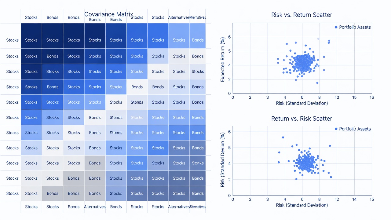
A covariance matrix quantifies how asset returns co-vary, forming the foundation for risk calculations in MPT. Construction begins with collecting time-series return data for each asset class. The formula for covariance between two assets i and j is Cov(R_i, R_j) = E[(R_i - μ_i)(R_j - μ_j)]. For multi-asset portfolios, this expands into an n-by-n matrix. In 2026 applications, analysts blend historical observations with forward-looking estimates derived from macroeconomic forecasts to capture shifting correlations during periods of inflation or recession signals.

Incorporating Real-World Constraints Like Transaction Costs

Pure theoretical MPT often overlooks practical frictions including brokerage fees, bid-ask spreads, taxes, and liquidity limits. To address these, optimization models add penalty functions or constraints that penalize excessive turnover. For instance, incorporating a transaction cost term reduces the attractiveness of frequent rebalancing. This produces allocations more aligned with actual 2026 market execution realities and helps preserve net returns over multi-year horizons.

Software Tools for Portfolio Optimization

Investors rely on accessible software to implement MPT calculations efficiently. Python libraries such as PyPortfolioOpt and SciPy enable mean-variance optimization with custom constraints. R users benefit from packages like PortfolioAnalytics for robust frontier generation. Spreadsheet applications with add-ins provide entry-level options, while institutional platforms offer advanced scenario modeling. Integrating live market feeds ensures models stay current with 2026 price movements and correlation shifts.

Practical Examples with Sample Portfolios

Consider a diversified sample portfolio initially allocated as 55 percent global equities, 25 percent investment-grade bonds, 12 percent real estate investment trusts, and 8 percent commodities. Applying MPT optimization might shift weights to reduce risk while maintaining target returns around long-term averages. Analysts then compare pre-optimization standard deviation against the optimized version to quantify diversification gains. Multiple iterations with different risk tolerances illustrate how the efficient frontier guides decision-making in practice.

Comparing Theoretical Outputs vs. 2026 Market Conditions

Theoretical MPT assumes normally distributed returns and stable correlations, yet 2026 markets frequently exhibit fat tails and regime shifts from policy announcements or supply chain events. Stress testing via Monte Carlo simulations or historical scenario analysis reveals gaps between model predictions and realized outcomes. Investors adjust by applying shrinkage estimators to covariance inputs or layering in black swan protections, yielding more resilient portfolios.

Steps for Implementation

1. Clearly define investment objectives, time horizon, and maximum acceptable drawdown levels.
2. Gather clean, high-quality return data from reliable sources spanning multiple market cycles.
3. Estimate key parameters including expected returns, variances, and the full covariance matrix, blending history with forward views.
4. Incorporate constraints such as position limits, sector exposures, and transaction cost adjustments into the optimization routine.
5. Generate the efficient frontier and select the portfolio matching the desired risk-return profile.
6. Backtest the chosen allocation against out-of-sample periods and implement through low-cost vehicles.
7. Establish a monitoring schedule for periodic rebalancing when drifts exceed predefined thresholds.

Advanced Techniques and Risk Management

Beyond basic mean-variance optimization, 2026 practitioners explore extensions such as Black-Litterman models that blend market equilibrium returns with investor views. Risk budgeting approaches allocate risk contributions evenly across assets rather than capital weights. Regular stress testing against interest rate spikes or equity crashes ensures portfolios withstand unexpected shocks common in the current decade.

Common Pitfalls and FAQ

Q: How should estimation errors in expected returns be handled? Apply robust optimization methods or use equilibrium-based models to dampen sensitivity to noisy inputs.

Q: What happens when asset correlations spike during crises? Re-estimate the covariance matrix frequently and run scenario analyses that simulate correlation breakdowns.

Q: Can MPT accommodate ESG constraints? Yes, by adding screening rules or tilt factors within the optimization framework without sacrificing core efficiency goals.

Q: How often should portfolios be rebalanced? Review allocations quarterly or when deviations exceed five percent of target weights, balancing cost against drift risk.

For deeper reading on portfolio construction fundamentals, consult resources from Investopedia, regulatory guidance at SEC.gov, and macroeconomic data from FederalReserve.gov.

Conclusion

Successfully applying Modern Portfolio Theory in 2026 demands rigorous data handling, realistic constraint integration, and continuous adaptation to market realities. By mastering efficient frontier analysis, covariance construction, and practical implementation steps, investors position themselves for superior risk-adjusted performance and lasting diversification benefits across asset classes.