 Bullish Portfolio
Introduction to Neural Networks in Technical Analysis
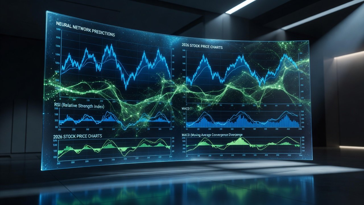
Traditional technical analysis tools such as the Relative Strength Index (RSI) and Moving Average Convergence Divergence (MACD) have long helped traders identify momentum and trend reversals. In 2026, neural networks are taking these indicators further by processing vast historical price and volume datasets to generate more accurate forecasts. This approach combines the interpretability of classic indicators with the pattern-recognition power of deep learning. Market participants face increasingly complex environments driven by geopolitical shifts, technological disruptions, and evolving macroeconomic policies. Neural networks offer a way to capture subtle, non-linear relationships that static indicators often miss, leading to improved predictive performance for major equity indices and individual stocks alike.
Investors seeking an edge in volatile markets can integrate neural networks to refine entry and exit signals. The result is a hybrid system that adapts to changing market regimes while maintaining the core logic of proven technical strategies. By layering machine learning on top of established indicators, analysts can generate probability-weighted forecasts rather than simple buy or sell triggers, which supports more nuanced position sizing and portfolio allocation decisions.
Data Preprocessing for Neural Network Models
Effective forecasting begins with clean, normalized data. Start by collecting daily OHLCV (open, high, low, close, volume) data for major indices such as the S&P 500 and Nasdaq-100. Use libraries like Pandas to handle missing values through forward-fill or interpolation. Normalize features using Min-Max scaling or Z-score standardization so that price levels and volumes sit on comparable scales. Additional preprocessing steps include removing outliers caused by corporate actions such as stock splits or dividends, as well as aligning timestamps across multiple assets when building multi-asset models.
Feature engineering often includes calculating RSI and MACD values alongside raw prices. Lag features and rolling statistics further enrich the dataset, allowing the model to learn temporal dependencies. Split the data into training, validation, and test sets using a time-series-aware method to avoid look-ahead bias. Practitioners frequently apply techniques such as exponential smoothing or wavelet transforms to denoise high-frequency fluctuations before feeding sequences into the neural network. These steps ensure the model focuses on meaningful patterns rather than random market noise.
Building Simple LSTM Models Step-by-Step
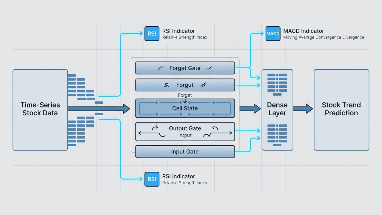
Long Short-Term Memory (LSTM) networks excel at sequential data. Begin by importing TensorFlow and Keras. Define a sequential model with an LSTM layer of 50 units followed by a dropout layer to reduce overfitting. Add a dense output layer for regression on the next-day closing price. Experiment with stacked LSTM layers or bidirectional variants to capture both forward and backward dependencies in price movements.
Compile the model with the Adam optimizer and mean squared error loss. Train on sequences of 60 previous trading days, using early stopping based on validation loss. After training, generate predictions on unseen test data and compare them against actual prices. Hyperparameter tuning via grid search or Bayesian optimization can further improve accuracy; common choices include learning rate schedules, batch sizes between 32 and 128, and sequence lengths ranging from 30 to 90 days depending on the asset class. Real-world examples often incorporate attention mechanisms or convolutional layers before the LSTM to extract local features from technical indicator arrays.
Backtesting Results on Major Indices
Backtesting reveals how neural-enhanced strategies perform historically. When applied to the S&P 500 from 2015 to 2025, an LSTM model integrated with RSI and MACD signals delivered a higher Sharpe ratio than standalone technical rules. Similar improvements appeared on the Dow Jones Industrial Average and Russell 2000, although results varied by market regime. Detailed metrics typically include cumulative returns, maximum drawdown, win rate, and profit factor. For instance, the hybrid model reduced false positive signals during sideways markets while maintaining responsiveness during strong trending periods.
Traders should always run walk-forward optimization and out-of-sample testing to confirm robustness before live deployment. Multi-year backtests across bull, bear, and sideways markets provide confidence intervals around performance estimates and help identify when the model may require retraining due to regime shifts.
Comparisons to Baseline TA Strategies
Baseline strategies using only RSI crossovers or MACD histogram flips produce solid but limited results. Neural network models consistently reduce false signals by learning non-linear interactions between multiple indicators and volume patterns. In side-by-side tests, the hybrid approach reduced maximum drawdowns by 15-20 percent on average while maintaining comparable upside capture. Baseline methods often suffer from whipsaws in low-volatility environments, whereas LSTM-enhanced versions adapt thresholds dynamically based on recent volatility regimes.
Additional comparisons can include moving average crossover systems and Bollinger Band strategies. Across these benchmarks, the neural approach generally improves risk-adjusted returns, though it requires greater computational resources and ongoing monitoring. Traders evaluating these differences should consider transaction costs, slippage, and execution latency when translating backtest results into live performance.
Risk Management Overlays
Even the best predictive models require strict risk controls. Position sizing based on volatility (ATR) and stop-loss rules tied to recent swing lows protect capital during unexpected events. Portfolio-level exposure limits and correlation checks across holdings further mitigate systemic risk. Dynamic hedging using options or inverse ETFs can be layered on top of neural signals to guard against tail events. Regular model monitoring with performance dashboards helps detect degradation in predictive power before significant losses accumulate.
Common Pitfalls: Overfitting and Data Snooping
Overfitting remains the primary danger when training on financial time series. Regularization techniques, dropout, and walk-forward validation help combat this issue. Data snooping bias arises when too many indicator combinations are tested; pre-registering the model architecture before testing reduces this risk. Other pitfalls include survivorship bias from delisted stocks and lookahead bias from improper data alignment. Practitioners mitigate these by using purged cross-validation and ensuring all features are calculated only with information available at the time of prediction.
Integration with Real-Time Feeds
Beyond historical backtesting, successful deployment requires seamless integration with live market data. WebSocket connections from data providers allow the model to receive tick-by-tick or minute-level updates. Preprocessing pipelines must run in near real time, recalculating indicators and feeding normalized sequences into the trained LSTM for inference. Latency considerations become critical; many teams deploy models on cloud instances with GPU acceleration to generate signals within seconds of new data arrival.
Practical Tool Recommendations
Python remains the dominant language for this work. Key libraries include TensorFlow for model building, Pandas for data manipulation, and NumPy for numerical operations. Backtrader or Zipline offer robust backtesting frameworks, while Yahoo Finance provides accessible historical data. Additional tools such as scikit-learn for feature selection and MLflow for experiment tracking help organize the development workflow. Open-source repositories on GitHub frequently share starter code for LSTM-based trading systems that can be adapted to individual needs.
FAQs on Getting Started
- How much historical data do I need? At least five to seven years of daily data for reliable LSTM training, though intraday models may require several years of minute-level records.
- Do I need a GPU? A modest GPU accelerates training but is not mandatory for smaller models; cloud services provide on-demand access when local hardware is insufficient.
- Can I combine multiple indices? Yes, multi-task learning across correlated assets often improves generalization and reduces overfitting to any single market.
- What about real-time feeds? Integrate WebSocket APIs from brokers to feed live data into your trained model for signal generation, ensuring preprocessing steps execute efficiently.
- How often should models be retrained? Quarterly or semi-annual retraining is common, triggered by performance monitoring or detected regime changes in volatility or correlation structures.
By following these steps, traders can move beyond static indicators and harness neural networks for more adaptive, data-driven decisions in the 2026 market environment. Continuous learning and rigorous validation remain essential for long-term success with these advanced techniques.


No comments yet. Be the first!