Monte Carlo Simulations for 2026 Asset Allocation

Introduction to Monte Carlo Simulations in Portfolio Management

Investors navigating 2026 market uncertainties need robust quantitative tools to optimize asset allocation. Monte Carlo simulations provide a powerful method for modeling portfolio outcomes by running thousands of random scenarios based on historical data and volatility assumptions. Unlike deterministic models that rely on single-point estimates, these simulations generate probability distributions that help assess risk and refine diversification strategies.

This guide covers the fundamentals, practical implementation using accessible tools, and advanced techniques for interpreting results. By the end, you will understand how to apply these methods to build resilient portfolios.

Fundamentals of Monte Carlo Simulations

Monte Carlo methods use repeated random sampling to estimate possible future states. In asset allocation, key inputs include expected returns, standard deviations, and correlations between asset classes. The output reveals the range of potential portfolio values, highlighting downside risks and upside opportunities.

These simulations excel in capturing non-linear relationships and fat-tail events common in financial markets, offering a more realistic view than traditional mean-variance optimization alone.

Step-by-Step Setup Using Python or Excel

Implementing Monte Carlo simulations starts with data collection. Gather historical returns for equities, bonds, and alternatives from reliable sources.

Python Implementation

Python offers flexibility through libraries like NumPy and Pandas. Begin by defining asset parameters, then simulate thousands of paths:

import numpy as np
np.random.seed(42)
num_simulations = 10000
portfolio_returns = []
for i in range(num_simulations):
    # Sample returns based on means and cov matrix
    sim_return = np.random.multivariate_normal(means, cov_matrix)
    portfolio_returns.append(np.dot(weights, sim_return))

Run the code to generate a distribution of ending portfolio values.

Excel Approach

For spreadsheet users, use RAND() functions combined with NORM.INV to model returns. Create columns for each asset class and drag formulas across 5,000+ rows to approximate simulations.

NumPy documentation provides detailed guidance on multivariate sampling techniques essential for accurate modeling.

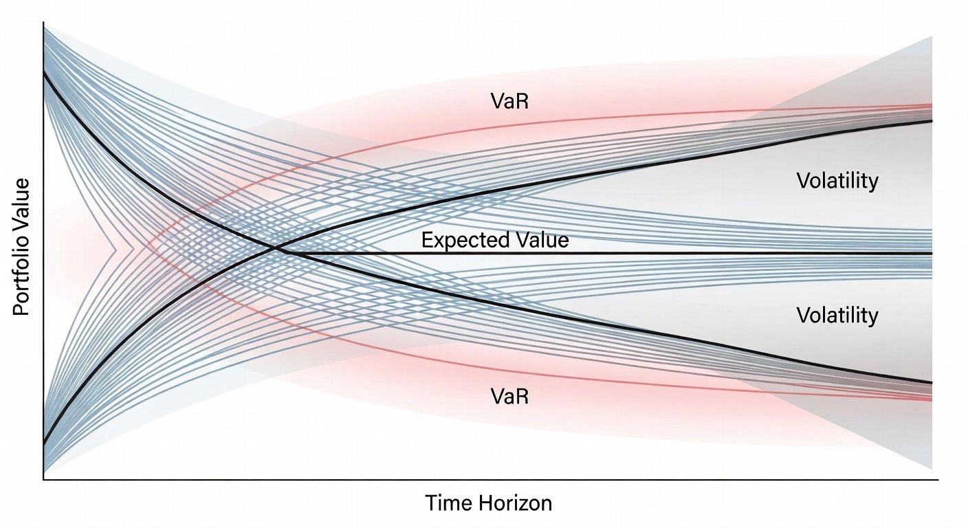
Interpreting Probability Distributions for Risk Assessment

Once simulations complete, analyze the resulting histogram or density plot. Key metrics include Value at Risk (VaR), Conditional VaR, and the probability of meeting retirement goals. For example, a 5% VaR shows the loss threshold exceeded only 5% of the time.

Compare median outcomes against worst-case scenarios to balance growth and protection.

Optimizing Allocations and Practical Examples

Run simulations across different weight combinations to identify efficient frontiers. A diversified portfolio with 60% equities and 40% bonds might show a 75% probability of positive returns over five years, versus 65% for a pure equity benchmark.

Sensitivity analysis involves shocking inputs like inflation spikes or correlation breakdowns to test robustness. This reveals how allocations perform under 2026-specific stresses such as geopolitical tensions.

Comparisons to Deterministic Models and Limitations

Deterministic forecasts provide a single expected path but ignore variability. Monte Carlo outputs deliver confidence intervals, making them superior for decision-making. However, results depend heavily on input assumptions—garbage in, garbage out.

FAQ

What assumptions matter most? Accurate volatility and correlation estimates drive reliability.
How many simulations are enough? 10,000 runs typically stabilize distributions for most portfolios.
Can Excel handle large runs? Yes, but Python scales better for complex multi-asset models.

Investopedia offers further reading on simulation validation techniques.