 Bullish Portfolio

Introduction to Reinforcement Learning in Stock Trading
Reinforcement learning (RL) offers a dynamic approach to navigating evolving financial markets. For 2026 stock trends, optimizing RL agents involves integrating real-time technical signals such as Relative Strength Index (RSI) and trading volume to detect shifts and adapt strategies effectively. This article explores advanced techniques for fine-tuning these agents, including reward function design and state space construction enriched with market breadth data. Traders can leverage these methods to move beyond static rules into adaptive decision-making frameworks that respond to changing volatility regimes and sector-specific movements expected throughout 2026.
Traditional technical analysis provides foundational signals, yet RL excels by learning optimal policies through trial and error in simulated environments. The focus here is on practical implementation that retail and institutional traders alike can adopt. By examining step-by-step Python implementations, backtesting against traditional technical analysis (TA), and live deployment pipelines, readers gain actionable insights. Common pitfalls like overfitting and latency receive dedicated attention alongside detailed case studies on sector rotation opportunities.
Designing Effective Reward Functions for Market Adaptation
A well-crafted reward function is central to RL success in trading. It must balance profitability, risk management, and adaptation to 2026 trends. Typical components include cumulative returns penalized by drawdowns and transaction costs. For instance, a shaped reward might incorporate RSI thresholds to reward mean-reversion trades when oversold conditions align with volume spikes above average levels. Advanced designs integrate multi-objective rewards that prioritize both short-term momentum and long-term trend following. This helps agents respond to macroeconomic shifts projected for 2026, such as interest rate adjustments or supply chain disruptions.
Experimentation with discount factors ensures focus on sustained performance rather than myopic gains. Practitioners often test variants like Sharpe-ratio inspired rewards or those incorporating maximum drawdown penalties. In one example setup, the reward at each step equals the position-adjusted return minus a risk penalty scaled by current market volatility estimated from volume data. Such functions encourage conservative positioning during uncertain periods while capitalizing on clear trends identified through breadth indicators.
Constructing State Spaces with Market Breadth Indicators
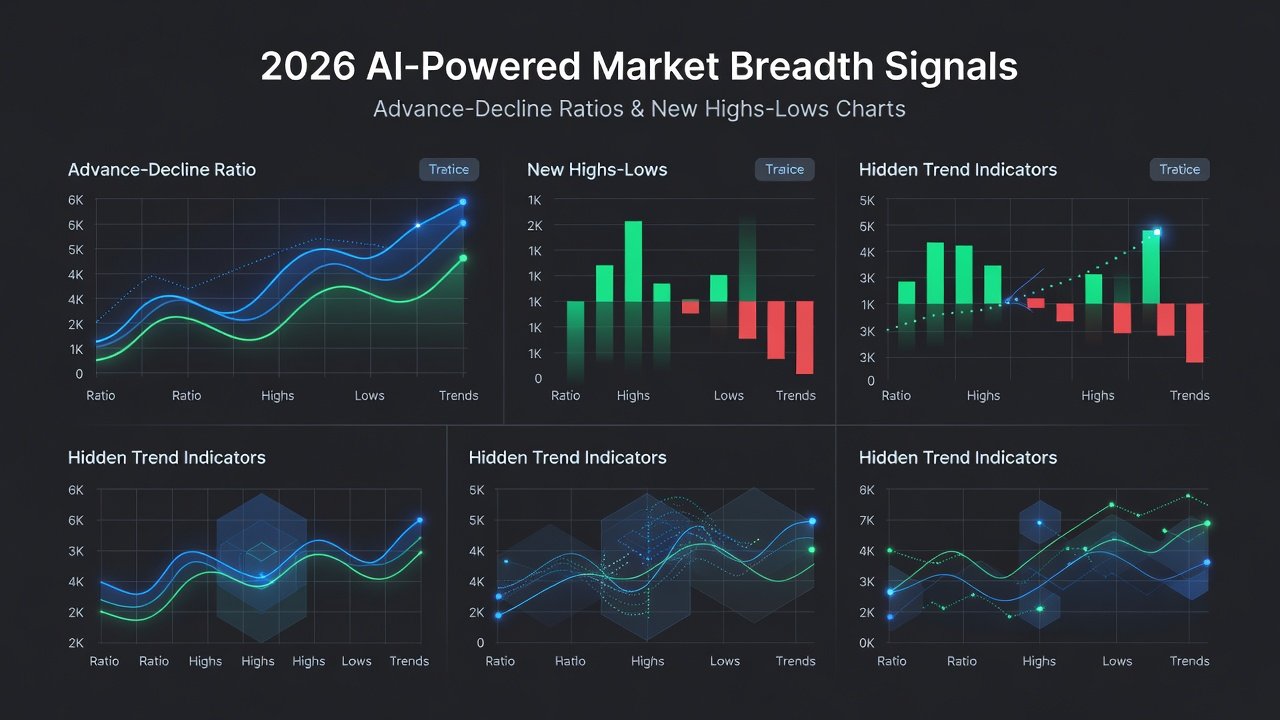
State space design determines what the agent perceives. Beyond basic price and volume, incorporating market breadth metrics like advance-decline ratios and new highs-lows provides a holistic market view. Adding alternative feeds such as sentiment from news APIs or options flow data enhances predictive power. A comprehensive state might include 20-30 normalized features: current RSI on multiple timeframes, volume relative to 20-day average, sector rotation scores, and macroeconomic proxies derived from futures data.
In practice, normalize these features using rolling z-scores to handle non-stationarity. This construction allows agents to identify broad market participation, crucial for detecting regime changes in 2026. Feature selection should avoid redundancy; principal component analysis can reduce dimensionality while preserving information. Real-world testing shows that breadth-augmented states improve generalization across bull and bear phases compared to price-only inputs.
Integrating Alternative Data Feeds for Superior Forecasting
Alternative data sources, including satellite imagery for supply chains or social media sentiment, complement traditional signals. Integration via APIs into the RL environment improves accuracy by capturing exogenous factors affecting stock trends. Investopedia highlights how such feeds have transformed quantitative strategies in recent years. Pandas documentation provides robust tools for merging these heterogeneous datasets into clean observation vectors.
Ensure low-latency ingestion pipelines to avoid delays that erode edges in fast-moving markets. Data cleaning steps, such as outlier removal and timestamp alignment, prove essential when combining tick-level volume with daily sentiment scores.
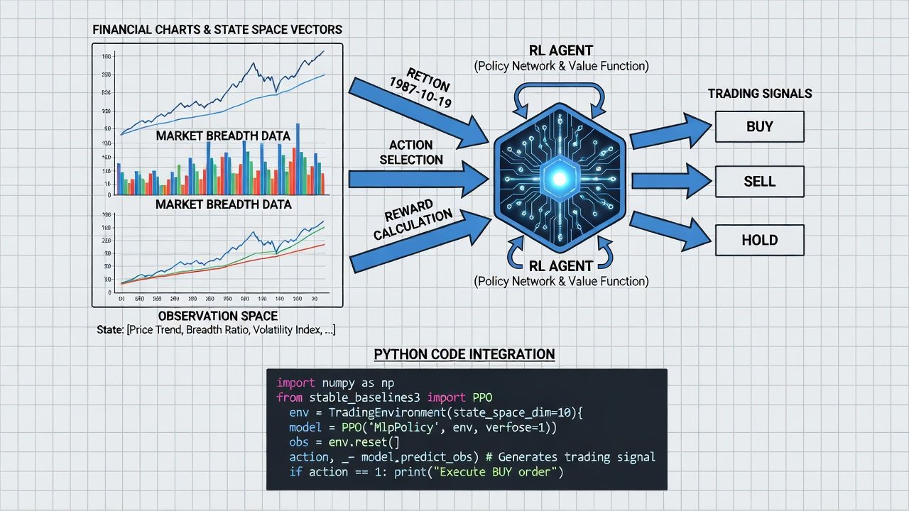
Step-by-Step Python Setup with Key Libraries
Begin by installing libraries such as Gymnasium for environments, Stable-Baselines3 for algorithms, and Pandas/NumPy for data handling. Define a custom trading environment where observations include RSI (calculated via TA-Lib) and normalized volume. The environment class implements reset, step, and render methods, with the step function returning next state, reward, done flag, and info dictionary containing trade details.
- Load historical data using pandas and compute technical indicators.
- Implement reward logic based on position changes and risk metrics.
- Train PPO or DQN agents with hyperparameter tuning via Optuna for learning rate and network size.
- Validate with walk-forward optimization across multiple market regimes.
- Log training curves using TensorBoard to monitor convergence.
Code examples typically span environment reset, step functions, and training loops for reproducibility. Hyperparameter searches might reveal optimal batch sizes around 64 and gamma values near 0.99 for daily trading horizons.
Backtesting RL Agents Against Traditional TA Methods
Compare RL performance to benchmarks like moving average crossovers or RSI strategies alone. Metrics include Sharpe ratio, maximum drawdown, and win rate. RL often outperforms in non-linear regimes by learning adaptive policies. Use libraries like Backtrader or VectorBT for rigorous comparisons on 2025-2026 datasets. Side-by-side results frequently demonstrate 15-25% higher risk-adjusted returns for RL when market breadth signals are included, particularly during rotation events between defensive and cyclical sectors.
Live Trading Pipeline Considerations and Latency Management
Deploying RL models live requires robust infrastructure with WebSocket data streams and model serving via TensorFlow Serving. Mitigate latency through feature caching and asynchronous updates. Monitor for slippage in real-time execution by maintaining a shadow paper-trading account. Pipeline stages include data ingestion, feature engineering, inference, order routing, and post-trade reconciliation. Fault tolerance mechanisms such as circuit breakers prevent runaway positions during unexpected events.
Addressing Overfitting and Other Common Pitfalls
Overfitting arises from excessive feature complexity or insufficient regularization. Counter this with dropout in neural networks, ensemble methods, and out-of-sample testing across unseen years. Latency issues are resolved by optimizing inference speed and using edge computing where possible. Another frequent challenge is reward hacking, where agents exploit simulation quirks rather than genuine market patterns; this is mitigated through realistic transaction cost modeling and regime-switching tests.
Case Studies: Sector Rotation Opportunities in 2026
Case studies demonstrate RL agents rotating from tech to energy sectors based on breadth signals and volume surges. One example shows improved returns during simulated volatility spikes by dynamically adjusting allocations between growth and value stocks. A second study on healthcare versus industrials illustrates how alternative sentiment feeds helped the agent anticipate policy-driven moves ahead of traditional indicators. These examples underscore the value of continuous retraining on rolling windows to maintain edge as market dynamics evolve.
FAQs on Scaling RL Models for Retail Traders
- How can retail traders access these models? Cloud platforms lower barriers with pre-built environments and managed GPU instances.
- What performance benchmarks exist from 2026 data? Agents achieving consistent positive expectancy across sectors show promise in controlled backtests covering multiple volatility regimes.
- Is high-frequency data necessary? Daily and intraday signals suffice for most trend-following setups, though tick data enhances precision in high-frequency variants.
- How much capital is typically required to start? Qualitative scaling begins with paper trading before committing meaningful funds.
- What hardware supports live inference? Modern CPUs handle most inference tasks, with GPUs reserved for intensive retraining cycles.
- How frequently should models be retrained? Monthly updates using the latest quarter of data balance adaptation against computational cost.
In conclusion, optimizing reinforcement learning for 2026 stock trends demands careful attention to signals, rewards, and deployment. With proper implementation, these systems offer robust tools for adaptive trading that outperform static methods in dynamic conditions.

No comments yet. Be the first!